Academic Factor Evaluation Guide (AcaEvaluatorModel & AcaIndirectEvaluator)
1. What is AcaEvaluatorModel?
AcaEvaluatorModel tests the explanatory/predictive power of academic (or self-built) factors on stock returns. It connects factor portfolio time series with individual stocks’ excess returns, and provides:
- Time-series regressions (Rolling/Expanding): obtain per-period coefficients, intercept (α), and statistics;
- Cross-sectional regressions: run a cross-sectional regression at each timestamp to examine the exposure–return relation;
- Fama-MacBeth regressions: two-step estimation of cross-sectional prices, producing mean β and t-statistics;
- Parallelization and sliding window control, suitable for mid-sized panels (Time × Stock).
Classic workflow (copy-paste ready)
# 1) Base data
from firefin.data.gateway import fetch_data
import pandas as pd
import numpy as np

data = fetch_data(['market_cap','return_adj','pb_ratio','open','close','volume'])
rf   = pd.read_feather('path/to/us_bond_2y.feather')  # Example risk-free rate

# 2) Select sample and derive indicators
mkt_cap = data['market_cap'].iloc[50:470, :100]
ret_adj = data['return_adj'].iloc[50:470, :100]
pb      = data['pb_ratio'].iloc[50:470, :100]
bm      = 1 / pb

# Align risk-free rate and build excess returns
rf = (rf.set_index('datetime') if 'datetime' in rf.columns else rf)
rf = rf['us_bond_2y']; rf.index = pd.to_datetime(rf.index).normalize()
rf = rf.reindex(mkt_cap.index.normalize(), method='ffill') / 100
rf.index = mkt_cap.index
risk_free_rate = rf
excess_ret = ret_adj.sub(risk_free_rate, axis=0).fillna(0)

# 3) Example: use PB for univariate sorting and take H−L as the factor portfolio
from firefin.core.algorithm.portfolio_sort import PortfolioSort
forward_returns = {0: ret_adj}
pb_quantile_ret = PortfolioSort.single_sort(
    factor=pb, forward_returns=forward_returns, quantiles=5, market_cap=mkt_cap
)
# Take H−L and wrap as list[pd.Series]
pb_HML = [pb_quantile_ret[0].iloc[:, -1]]

from firefin.evaluation.academia.AcaEvaluatorModel import AcaEvaluatorModel

model = AcaEvaluatorModel(
    factor_portfolio = pb_HML,     # list[pd.Series]
    return_adj       = excess_ret, # Time × Stock
    n_jobs           = 10,         # number of parallel workers
    time_series_window = None,     # pass None; set a window size here if you need rolling tests
    all_time_series_regression = True, # True=single full-sample regression; False=sliding window
    verbose          = 1,
)

# 1) Time-series regression: rolling coefficients/intercept/residuals/statistics
ts_res = model.run_time_series_regression(fit_intercept=True)

# 2) Cross-sectional regression: explain stock returns each period
cs_res = model.run_cross_sectional_regression()

# 3) Fama-MacBeth: two-step estimation of cross-sectional prices
fm_res = model.run_fama_macbeth_regression()
2.1 Required inputs
factor_portfolio: list[pd.Series]A set of time series of factor portfolio returns (e.g., H−L, market factor, size factor, etc.). EachSeriesis indexed by date, and its length must equal the number of rows inreturn_adj.return_adj: pd.DataFrameThe matrix of individual stock returns, with shape Time × Stock. Index = dates, columns = stock tickers.
- Use
PortfolioSort.single_sort(...)to obtain quantile portfolio returns, then take the H−L column to form thepb_HMLlist;- Subtract the risk-free rate from individual stock returns to get excess returns
excess_ret;- Feed both into
AcaEvaluatorModel:basic_test = AcaEvaluatorModel( factor_portfolio = pb_HML, # list[pd.Series] return_adj = excess_ret # Time × Stock DataFrame )
2.2 Indexing & missing-value conventions
- Date indexes must be perfectly aligned (same frequency, no duplicates). It’s recommended to pre-handle missing values (
dropna/ forward-fill / mask columns). - If trading halts / IPOs within the window cause NaNs, the model will treat NaNs as 0 after ingestion.
Data preparation example:
# 1) Base data
from firefin.data.gateway import fetch_data
import pandas as pd
import numpy as np

data = fetch_data(['market_cap','return_adj','pb_ratio','open','close','volume'])
rf   = pd.read_feather('path/to/us_bond_2y.feather')  # Example risk-free rate

# 2) Select sample and derive indicators
mkt_cap = data['market_cap'].iloc[50:470, :100]
ret_adj = data['return_adj'].iloc[50:470, :100]
pb      = data['pb_ratio'].iloc[50:470, :100]
bm      = 1 / pb

# Align risk-free rate and build excess returns
rf = (rf.set_index('datetime') if 'datetime' in rf.columns else rf)
rf = rf['us_bond_2y']; rf.index = pd.to_datetime(rf.index).normalize()
rf = rf.reindex(mkt_cap.index.normalize(), method='ffill') / 100
rf.index = mkt_cap.index
risk_free_rate = rf
excess_ret = ret_adj.sub(risk_free_rate, axis=0).fillna(0)

# 3) Example: use PB for univariate sorting and take H−L as the factor portfolio
from firefin.core.algorithm.portfolio_sort import PortfolioSort
forward_returns = {0: ret_adj}
pb_quantile_ret = PortfolioSort.single_sort(
    factor=pb, forward_returns=forward_returns, quantiles=5, market_cap=mkt_cap
)
# Take H−L and wrap as list[pd.Series]
pb_HML = [pb_quantile_ret[0].iloc[:, -1]]
- Evaluation
Goal: Use the pb_HML factor portfolio to explain individual stocks’ excess returns excess_ret.
from firefin.evaluation.academia.AcaEvaluatorModel import AcaEvaluatorModel

model = AcaEvaluatorModel(
    factor_portfolio = pb_HML,     # list[pd.Series]
    return_adj       = excess_ret, # Time × Stock
    n_jobs           = 10,         # number of parallel workers
    time_series_window = None,     # pass None; set a window size here if you need rolling tests
    all_time_series_regression = True, # True=single full-sample regression; False=sliding window
    verbose          = 1,
)

# 1) Time-series regression: rolling coefficients/intercept/residuals/statistics
ts_res = model.run_time_series_regression(fit_intercept=True)

# 2) Cross-sectional regression: explain stock returns each period in the cross section
cs_res = model.run_cross_sectional_regression()

# 3) Fama-MacBeth: two-step estimation of cross-sectional prices
fm_res = model.run_fama_macbeth_regression()
Regression result objects typically include: coefficients, intercept (α), residuals, standard errors, t-stats, and R².
# Accessing model outputs
ts_res.beta     # factor exposures from time-series regressions
ts_res.tvalue   # t-stats for factor exposures
ts_res.alpha    # intercept from time-series regressions
ts_res.alpha_t  # t-stat for the intercept
ts_res.r2       # R^2
- API details (function I/O + tunable parameters)
This section clarifies the constructor and the three regression methods—their inputs, outputs, defaults, and constraints—and shows how to set parameters such as a custom time window.
4.1 Constructor AcaEvaluatorModel(...)
Signature
AcaEvaluatorModel(
    factor_portfolio: list[pd.Series],
    return_adj: pd.DataFrame,
    n_jobs: int = 10,
    time_series_window: int = 60,
    all_time_series_regression: bool = True,
    verbose: int = 0,
    cov_type = None,
)
Parameter descriptions
| Parameter | Type/Shape | Default | Purpose | Constraints/Notes | Typical values/Advice |
|---|---|---|---|---|---|
| factor_portfolio | list[pd.Series]; each Series indexed by date with length = T (sample size). K = #factors. | Required | Provide time-series returns of factor portfolios (e.g., H−L, MKT, SMB …). Internally each factor is duplicated across return_adj’s columns to run regressions. | Each Series must have the same #rows as return_adj; index (dates) must align with return_adj.index; pre-handle missing values if possible. | If only 1 factor, still wrap in a list, e.g., [hml_series]. |
| return_adj | pd.DataFrame, shape = T × N (Time × Stock). | Required | Dependent variable: usually individual stocks’ excess returns (risk-free already subtracted). | Columns are tickers/IDs; index must fully align with all factors; consider handling missing or dropping columns with too many NaNs. | Use a single frequency (daily/weekly/monthly). |
| n_jobs | int | 10 | Parallelism for batched regressions (time-series / cross-sectional / FM). | Constrained by CPU cores & memory; parallel backends may vary across platforms. | Set to logical CPU count or slightly below. |
| time_series_window | int | 60 | Rolling window length. Only effective when all_time_series_regression=False. | If all_time_series_regression=True, the internal window becomes full sample length T; this parameter is ignored. | For monthly data 36 (3y); for daily 252, 504, etc. |
| all_time_series_regression | bool | TRUE | Whether to run a single full-sample time-series regression. | Set False to enable time_series_window for rolling regressions. | Use False for stability/time-varying analyses. |
| verbose | int | 0 | Logging verbosity. | 1 or 2 prints more progress. | Increase for debugging, lower for production. |
| cov_type | str | None | Covariance kernel type | None: standard i.i.d. residual assumption for t-stats; HAC: Newey-West t-statistics. |
4.2 Time-series regression run_time_series_regression(fit_intercept: bool = True, window = self.window, cov_type = self.cov_type)
# 1) Time-series regression: rolling coefficients/intercept/residuals/statistics
ts_res = model.run_time_series_regression(fit_intercept=True)
Inputs
fit_intercept: bool = True: whether to estimate the intercept (α).window: int = 60: regression window size.cov_type: str = None: which covariance kernel to use.
Outputs/Return
- Returns and saves to
self.time_series_res: a batched time-series regression result object fromRollingRegressor. - Exact fields depend on implementation; common ones (subject to implementation):
coef/beta(per time × per factor × per stock, or aggregated);intercept/alpha,stderr,tvalue/pvalue,r2,resid;- Possible exporters:
to_frame()/to_xarray()/summary().
Custom window
- Control via the constructor:
# Full-sample once:
AcaEvaluatorModel(..., all_time_series_regression=True)
# Rolling 120 periods:
AcaEvaluatorModel(..., all_time_series_regression=False, time_series_window=120)
Usage tips
- Check whether
alphasignificantly deviates from 0; - Examine stability of rolling
beta; - Beware multicollinearity among highly correlated factors; using kernel type
"HAC"is recommended.
4.3 Cross-sectional regression run_cross_sectional_regression()
# 2) Cross-sectional regression: explain stock returns each period
cs_res = model.run_cross_sectional_regression()
Inputs
- None (all dependencies come from the parameters set in
AcaEvaluatorModelinitialization, such astime_series_window,cov_type,fit_intercept).
What it does internally
- Calls
cross_sectional_regression(self.time_series_res, self.return_adj, window=self.time_series_window, skip_time_series_regression=True, n_jobs=self.n_jobs, verbose=self.verbose, cov_type = self.cov_type). - The typical flow uses individual stock exposures/loadings from the previous step as regressors at each time, and runs cross-sectional OLS on stock returns to obtain per-period coefficients and statistics.
Outputs/Return
BatchRegressionResult:- Contains per-timestamp cross-sectional coefficients,
intercept,stderr / tvalue / pvalue,R².
- Contains per-timestamp cross-sectional coefficients,
4.4 Fama-MacBeth regression run_fama_macbeth_regression()
# 3) Fama-MacBeth: two-step estimation of cross-sectional prices
fm_res = model.run_fama_macbeth_regression()
Inputs
- None (all dependencies come from the parameters set in
AcaEvaluatorModelinitialization, such astime_series_window,cov_type,fit_intercept).
What it does internally
- Calls
FamaMacBeth.run_regression(self.time_series_res, self.return_adj, window=self.time_series_window, skip_time_series_regression=True, n_jobs=self.n_jobs, verbose=self.verbose, cov_type = self.cov_type), executing the two-step procedure:- Obtain exposures from the time-series regression;
- Run cross-sectional regressions over time, and summarize average risk prices (λ) and their significance (common practice uses time-series-correlation-robust standard errors, e.g., Newey-West/HAC).
Outputs/Return
BatchRegressionResult(aggregated two-step results):- Average λ (risk prices) per factor, their
t/pvalues, and the significance of theintercept.
- Average λ (risk prices) per factor, their
5.1 Constructor AcaIndirectEvaluator.__init__(...)
Typical workflow (copy-paste ready)
from firefin.data.gateway import fetch_data
import pandas as pd
import numpy as np

data = fetch_data(['market_cap','return_adj','pb_ratio','open','close','volume'])
rf   = pd.read_feather('path/to/us_bond_2y.feather')  # Example risk-free rate

# 2) Select sample and derive indicators
mkt_cap = data['market_cap'].iloc[50:470, :100]
ret_adj = data['return_adj'].iloc[50:470, :100]
pb      = data['pb_ratio'].iloc[50:470, :100]
bm      = 1 / pb

# Align risk-free rate and build excess returns
rf = (rf.set_index('datetime') if 'datetime' in rf.columns else rf)
rf = rf['us_bond_2y']; rf.index = pd.to_datetime(rf.index).normalize()
rf = rf.reindex(mkt_cap.index.normalize(), method='ffill') / 100
rf.index = mkt_cap.index
risk_free_rate = rf
excess_ret = ret_adj.sub(risk_free_rate, axis=0).fillna(0)

# Build momentum signal
mom_signal = (data["close"] / data["close"].shift(21) -1).shift(1).iloc[50:470, :100]

# Example: use PB for univariate sorting and take H−L as the factor portfolio
from firefin.core.algorithm.portfolio_sort import PortfolioSort
forward_returns = {0: ret_adj}
pb_quantile_ret = PortfolioSort.single_sort(
    factor=pb, forward_returns=forward_returns, quantiles=5, market_cap=mkt_cap
)
# Take H−L and wrap as list[pd.Series]
pb_HML = [pb_quantile_ret[0].iloc[:, -1]]

from firefin.evaluation.academia.AcaIndirectEvaluator import AcaIndirectEvaluator
# Create AcaIndirectEvaluator
pb_HML_indirect_test = AcaIndirectEvaluator(factor_portfolio=pb_HML,
                                            return_adj=ret_adj,
                                            risk_free_rate=risk_free_rate,
                                                            stock_size=mkt_cap,
                                             stock_value=bm,
                                             mom_signal=mom_signal)
#  GRS robustness (window must be > N + K)
pb_HML_indirect_test.evaluate_stability(mode = "ff3_mom",window = 110)


from firefin.evaluation.academia.AcaIndirectEvaluator import *
# Build quantile returns
quantile_ret = [pb_quantile_ret[0][col] for col in pb_quantile_ret[0].columns]
# Create AcaIndirectEvaluator
indirect_test = AcaIndirectEvaluator(factor_portfolio=quantile_ret,
                                     return_adj=ret_adj,
                                     risk_free_rate=risk_free_rate,
                                     stock_size=mkt_cap,
                                     stock_value=bm,
                                     mom_signal=mom_signal)

# 1) Benchmark comparison (last-period α/β + adjusted R²)
indirect_test.evaluate_by_other_factors(mode = "ff3_mom")
# 2) Cumulative α trajectory (expanding window)
indirect_test.cumulated_alpha(mode = "ff3_mom")
# 3) One-click LaTeX table (includes CAPM, FF3+MOM, custom)
latex_str = indirect_test.export_evaluation_table()
Signature
AcaIndirectEvaluator(
    factor_portfolio: list[pd.Series],
    return_adj: pd.DataFrame,
    time_series_window: int = 60,
    all_time_series_regression: bool = True,
    *,
    risk_free_rate: pd.Series,
    stock_size: pd.DataFrame,                 # market cap (for size weighting / constructing benchmarks)
    stock_value: pd.DataFrame | None = None,  # book-to-market (BM)
    op: pd.DataFrame | None = None,           # operating profitability (RMW-related)
    ag: pd.DataFrame | None = None,           # asset growth / investment (CMA-related)
    mom_signal: pd.DataFrame | None = None,   # momentum signal
    n_jobs: int = 10,
    verbose: int = 0,
)
Parameters (only new/specific ones listed; others same as §4.1)
| Parameter | Type/Shape | Requirement | Purpose/Notes | Typical values/Notes |
|---|---|---|---|---|
| risk_free_rate | pd.Series (T×1) | Required | Risk-free rate; used to form excess returns and benchmark factors. Index aligned with data. | Same unit/frequency as return_adj (e.g., monthly). |
| stock_size | pd.DataFrame (T×N) | Required | Market cap time series; for constructing MKT/SMB and weights. | Align with return_adj; fill missing as needed. |
| stock_value | pd.DataFrame (T×N) | Depends on mode | BM values; required for mode=”ff3” or “ff3_mom” or “ff5”. | Can use 1/pb_ratio. |
| op | pd.DataFrame (T×N) | Required for ff5 | Profitability indicator (RMW-related). | Keep frequency/definitions consistent. |
| ag | pd.DataFrame (T×N) | Required for ff5 | Investment/asset growth (CMA-related). | Same as above. |
| mom_signal | pd.DataFrame (T×N) | Required for ff3_mom | Momentum signal; to construct WML/MOM factor. | Common choices: 12-1 or 6-1 momentum. |
Indexing requirement: All the above time indexes must fully align with
factor_portfolio/return_adj. Internally the implementation commonly usesfillna(0)for simplicity, but in practice, proper preprocessing is recommended.
5.2 Benchmark “modes” & factor bundles (bundle_*)
evaluate_by_other_factors / cumulated_alpha / evaluate_stability choose the pricing model via mode:
| mode | Meaning | Required inputs | Internal call | #factors k (example) |
|---|---|---|---|---|
| “capm” | CAPM (market factor) | risk_free_rate, stock_size | bundle_capm(…) | 1 (MKT) |
| “ff3” | Fama–French 3-factor | also needs stock_value | bundle_ff3(…) | 3 (MKT, SMB, HML) |
| “ff3_mom” | FF3 + Momentum | also needs stock_value, mom_signal | bundle_ff3_mom(…) | 4 (MKT, SMB, HML, MOM) |
| “ff5” | Fama–French 5-factor | also needs stock_value, op, ag | bundle_ff5(…) | 5 (MKT, SMB, HML, RMW, CMA) |
| “customize” | Custom factor set | needs factor2: list[pd.Series] | use factor2 directly | Determined by the passed factors |
If required inputs are missing, a
ValueErrorwill be raised (implemented in code). The.nameattribute of benchmark factor series will be used for result column names.
5.3 Method 1: evaluate_by_other_factors(...)
Purpose: For each portfolio return, run OLS (single full-sample) under the chosen mode, and return the last period’s coefficients, t-values, and adjusted R².
Signature & parameters
evaluate_by_other_factors(
    mode: Literal["capm","ff3","ff3_mom","ff5","customize"] = "capm",
    factor2: list[pd.Series] | None = None,
)
mode: see §5.2;factor2: required only whenmode="customize"; custom factor list (indexes must align; setnameattributes).
Return values
coefficient_df : pd.DataFrame   # [alpha, factor betas] for each portfolio at the *last period*
statistics_df  : pd.DataFrame   # [alpha_t, factor t-values] at the same period
r2_adj_series  : pd.Series      # adjusted R^2 for each portfolio’s regression (single full-sample)
# Row index: portfolio names (from self.factor_portfolio[i].name)
# Columns ordered as: ["alpha", *factor_names]
Core implementation points
- Stack chosen factors
customized_factor_listintox(shape approx.(k, T, 1)), and for each portfolioy, runRollingRegressor(...).fit(window=None)(i.e., a single full-sample regression). - Take
res.alpha.iloc[-1],res.beta.iloc[:,0].valuesas the “last period” coefficients; similarly obtainalpha_tandtvalue. - Adjusted R² computed manually: , where
nis sample size andkis #factors.
Example
coef, tval, r2a = indirect.evaluate_by_other_factors(mode="ff3_mom")
# Custom:
my_factors = [carry, value_signal, quality]; [f.rename(n) for f,n in zip(my_factors,["CARRY","VAL","QTY"])];
coef_c, tval_c, r2a_c = indirect.evaluate_by_other_factors(mode="customize", factor2=my_factors)
Interpretation
alphainsignificantly different from 0 ⇒ the portfolio return is well explained by the benchmark;- Significant
alpha≠ 0 ⇒ potential anomalies/omitted factors; - Larger
R²_adj⇒ stronger explanatory power; comparing modes (adding HML/MOM/RMW/CMA) shows whether α vanishes.
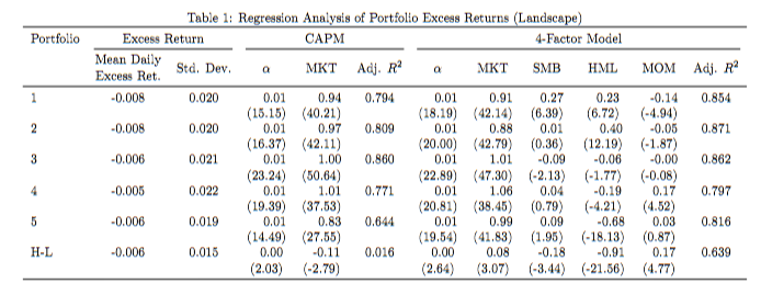
Regression coefficients:
         alpha       MKT
1     0.007082  0.944907
2     0.007462  0.965323
3     0.009172  1.004914
4     0.010420  1.013731
5     0.008710  0.832304
H-L   0.001629 -0.112603
t-statistics:
           alpha        MKT
1     15.150826  40.209226
2     16.366894  42.114703
3     23.239453  50.643657
4     19.391861  37.525036
5     14.493777  27.546402
H-L    2.031361  -2.793442
Radj2R^2_{adj}:
1      0.794081
2      0.808820
3      0.859527
4      0.770553
5      0.643951
H-L    0.015978
5.4 Method 2: cumulated_alpha(...)
Purpose: Expanding-window regressions over time to track the evolution of α as the sample grows; can plot or return the time series.
Signature & parameters
cumulated_alpha(
    mode: Literal["capm","ff3","ff3_mom","ff5","customize"] = "capm",
    factor2: list[pd.Series] | None = None,
    starting_point: int = 20,
    plt: bool = True,
)
starting_point: start estimating α once the sample size reaches this number (no estimates before it);plt: ifTrue, callplot_cumulative_alphato plot; ifFalse, returnlist[pd.Series](one α curve per portfolio, aligned with original dates).
Return values
plt=True: directly plots, no return;plt=False:list[pd.Series](Series name = portfolio name).
Implementation details
- For each
i = starting_point … T: take sample 0..i, run a full-sample regression (RollingRegressor(..., window=None)), and record the last-period α from that regression; - This yields the time series “α(i)”, i.e., the stability trajectory of α as the sample expands.
Interpretation
- If the α curve converges to 0 with decreasing volatility ⇒ the abnormal return weakens with a longer sample/more comprehensive benchmarks;
- If α stays stably positive/negative and significant ⇒ a more credible pricing anomaly or model omission.
5.5 Method 3: evaluate_stability(...) — Rolling GRS robustness
Purpose: Rolling robustness evaluation based on the GRS joint test. Tests whether, under given benchmark factor sets, the α of all tested assets (here, the stock cross section) are jointly zero.
Signature & parameters
evaluate_stability(
    value_weighted: bool = True,                 # not directly used for now; reserved for extensions
    mode: Literal["single","capm","ff3","ff3_mom","ff5"] = "single",
    window: int = 30,
    plt: bool = True,
)
mode="single": use only the “tested portfolio itself” as an explanatory variable (equivalent to testing whether this portfolio can explain individual stocks’ excess returns);- Other
modevalues: concatenate the chosen benchmark factors with the “tested portfolio”, and explain the stock excess returns together; - Window requirement:
window > N + K(the code checksmin_win = N + K + 1), whereN= number of stocks andK= #regressors (benchmark factors + #tested portfolios).
Return values
plt=True: returnsplot_grs_pval(grs_pval_series)(plot object);plt=False: returnspd.Seriesnamed"grs_pval"with date index (aligned, front-filled as needed).
Implementation notes
- Assemble regressors:
single⇒concat_return = factor_excess_ret(tested portfolio only);- otherwise ⇒
concat_return = factor_list + factor_excess_ret(benchmarks + tested portfolio).
- Use
RollingRegressor(window=window)to regress the stock excess return matrix, and obtain per-periodbetaandalpha; - Compute the GRS p-value in each rolling window: large p ⇒ fail to reject “α jointly zero”; small p ⇒ significant unexplained α remains.
Interpretation
- High p-values (e.g., >0.95, blue line in figure): benchmark + tested portfolio explain the stock-level returns well; joint α is insignificant;
- Low p-values: significant abnormal returns remain within that window ⇒ insufficient explanatory power or weak stability.
5.6 Method 4: export_evaluation_table(...) — One-click LaTeX table export
Purpose: Summarize return statistics and regression results (CAPM, FF3+MOM, optionally custom) into a single LaTeX table (for papers/reports).
Signature & parameters
export_evaluation_table(
    mode: str = "daily",                      # frequency: daily, monthly, yearly
    customized_factor: list[pd.Series] | None = None,
) -> str
Internal flow
- Compute each portfolio’s excess return
excess_ret = portfolio - risk_free_rateand summarize:summarize_returns; - Regressions:
mode="capm"results:mkt_df, mkt_stats_df, mkt_r2_adj;mode="ff3_mom"results:ff4_df, ff4_stats_df, ff4_r2_adj;- If
customized_factoris provided, runcustomizeas well;
- Use
stitch_coeff_tvalue(...)to combine coefficients + t-values into MultiIndex columns (two levels per column:(factor_name, coeff|tvalue)); - Call
latex_table(...)to produce the final LaTeX string and return it.
Return
str: write to.texor paste into your paper; includes:- Return statistics (mean/std);
alpha/βand their t-values for each model;R²_adjper model.
Other functions
AcademicFactors
This project provides convenient constructors for classic academic factors: ff3, ff5, ff3+mom, returning a list of [pd.Series] (the project’s standard factor structure).
from firefin.evaluation.academia.AcademicFactors import *
ff3 = bundle_ff3(stock_return = ret_adj,
    size = mkt_cap,
    book_to_market = bm,
    market_cap = mkt_cap,
    risk_free_rate = risk_free_rate)

ff5 = bundle_ff5(stock_return = ret_adj,
    size = mkt_cap,
    book_to_market = bm,
    market_cap = mkt_cap,
    profitability = profitability,
    investment = investment,
    risk_free_rate = risk_free_rate)

ff3_mom = bundle_ff3(stock_return = ret_adj,
    size = mkt_cap,
    book_to_market = bm,
    market_cap = mkt_cap,
    momentum_signal = momentum_signal,
    risk_free_rate = risk_free_rate)
For individual academic factors, the project also provides dedicated constructors:
# Market factor
mkt = market_excess(stock_return = ret_adj, size = mkt_cap, risk_free_rate = risk_free_rate)
# HML factor
hml = hml(stock_return = ret_adj, size = mkt_cap, book_to_market = bm)
# SMB factor (ff3 and ff5 versions slightly differ)
smb_ff3 = smb_ff3(stock_return = ret_adj, size = mkt_cap, book_to_market = bm)
smb_ff5 = smb_ff5(stock_return = ret_adj, size = mkt_cap, book_to_market = bm, profitablity = profitability, investment = investment)
# Momentum factor
mom = mom(stock_return = ret_adj, size = mkt_cap, momentum_signal = momentum_signal)
cross_sectional_regression
This project can run cross-sectional regressions on factors alone and return regression parameters.
from firefin.core.algorithm.cross_sectional_regression import *
xs=cross_sectional_regression(ff3, excess_ret,cov_type="HAC",window=50)
Here you can set the rolling window window as needed. cov_type specifies the method for computing t-statistics. cov_type=None gives standard OLS t-statistics; cov_type="HAC" computes Newey-West t-statistics.
Fama macbeth regression
This project can run standalone Fama-MacBeth regressions on factors and return regression parameters.
from firefin.core.algorithm.fama_macbeth import *
fm=FamaMacBeth.run_regression(ff3, excess_ret,window=50)
You can set the rolling window window here as well.