Evaluate Industrial Factor

Evaluation of Industrial Factors

Typical Workflow (copy-paste ready)

start_date = '2010-01-01'
end_date   = '2023-03-31'
#%%
# Load data
from firefin.data.gateway import *
data = fetch_data(["open", "close", "volume","return_adj"])

close_price = data["close"].loc[start_date:end_date]
open_price = data["open"].loc[start_date:end_date]
volume = data["volume"].loc[start_date:end_date]

#%%
# Compute forward returns for 1, 5, 10 days
from firefin.core.eva_utils import *
# compute forward returns
fr = compute_forward_returns(open_price.shift(-1), [1, 5, 10])
#%%
# Construct a factor (shown here just for demonstration; the factor format is a T×N pd.DataFrame)
def ts_corr(x, y, window=10):
    """
    Wrapper function to estimate rolling correlations.
    :param x, y: pandas DataFrames.
    :param window: the rolling window.
    :return: a pandas DataFrame with the time-series min over the past 'window' days.
    """
    return x.rolling(window).corr(y)

factor = ts_corr(close_price, volume, 20)
#%%
# Evaluator for industrial factors; it can evaluate the parameters of a new factor. This tool is not yet fully refined.
from firefin.evaluation.industry.evaluator import Evaluator
mng = Evaluator(factor, fr)
#%%
# Get the factor’s IC backtest data
df_ic = mng.get_ic("pearson")
#%%
# Get the factor’s quantile return backtest data
df_qr = mng.get_quantile_returns(5)

Step 0. Prepare Two Types of Data

Shape: both should be T×N pandas.DataFrames; rows are dates, columns are stocks (or industry constituents).
Date index: ideally a DatetimeIndex, but it’s fine if not—Evaluator will convert automatically.
Data: build a forward-return dictionary where the key is the holding period in days, and the value is the DataFrame of returns.

Example:

# Set the backtest period
start_date = '2019-01-01'
end_date   = '2023-03-31'
# Pull data
from firefin.data.gateway import fetch_data
data = fetch_data(["open", "close", "volume","return_adj"])
close_price = data["close"].loc[start_date:end_date]
open_price  = data["open"].loc[start_date:end_date]
return_adj  = data["return_adj"].loc[start_date:end_date]
# Build the forward return dictionary
from firefin.core.eva_utils import compute_forward_returns
# Note shift(-1): align the "next day’s open" to the signal day
fr = compute_forward_returns(open_price.shift(-1), [1, 5, 10])  # returns a dict: {1: df, 5: df, 10: df}

Step 1. Use `eva_utils` to Compute “Forward Returns” and Understand IC/Quantiles

eva_utils provides the low-level evaluation capabilities that Evaluator uses directly.

compute_forward_returns(price, periods): given adjusted prices, compute forward returns for 1/5/10 days.
compute_ic(factor, forward_returns, method): IC = cross-sectional correlation (most commonly Spearman, i.e., RankIC).
compute_quantile_returns(factor, forward_returns, quantiles): portfolio returns grouped by factor quantiles.
summarise_ic(ic): summarize IC mean/standard deviation/IR/proportions, etc., into a table.

Step 2. Prepare the Factor (T×N)

# Construct a factor (shown here just for demonstration; the factor format is a T×N pd.DataFrame)
def ts_corr(x, y, window=10):
    """
    Wrapper function to estimate rolling correlations.
    :param x, y: pandas DataFrames.
    :param window: the rolling window.
    :return: a pandas DataFrame with the time-series min over the past 'window' days.
    """
    return x.rolling(window).corr(y)

factor = ts_corr(close_price, volume, 20)

Step 3. One-Click Evaluation

Evaluator wraps the core capabilities of eva_utils into two out-of-the-box tasks—IC and quantile portfolio returns—and plots them automatically.

from firefin.evaluation.industry.evaluator import Evaluator
# Initialize the evaluator class; provide two parameters: the factor DataFrame `factor` and the factor’s forward returns `fr`
evaluator = Evaluator(factor, fr)

Get IC-related test metrics for this factor:

evaluator.get_ic(method="spearman", plot=True) 
# methods: Spearman/Kendall/Pearson; the most common is Spearman

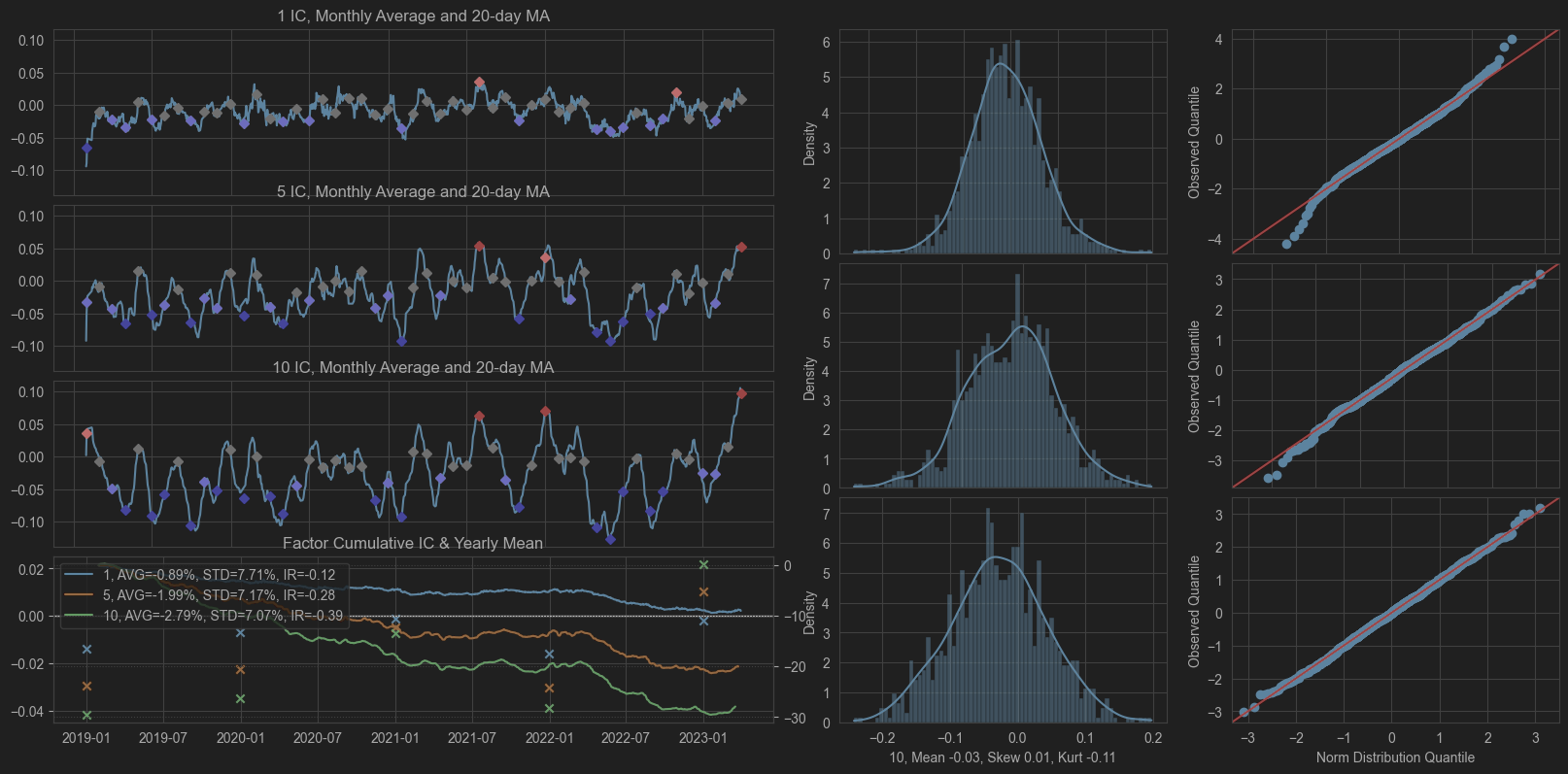
IC time series plots (the more stable the better; high IR, high proportion > 0; strong factors typically have average RankIC > 0).
Top-left three plots: 20-day moving averages of the IC between the factor values and the 1-, 5-, and 10-day forward returns.
Bottom-left plot: cumulative IC for 1/5/10 days, along with the IC mean, standard deviation, and IR (IC mean / standard deviation).
Middle three plots: distributions of IC values—top to bottom correspond to 1-, 5-, and 10-day ICs (the bottom of each shows the mean, kurtosis, and skewness).
Right-hand three plots: IC normality (values above the red line indicate probabilities exceeding those under a normal distribution in that region; if both tails are above, it suggests the IC may take more extreme values).

Get the factor’s grouped return series metrics:

# Get the factor’s quantile return backtest data
df_qr = evaluator.get_quantile_returns(5)

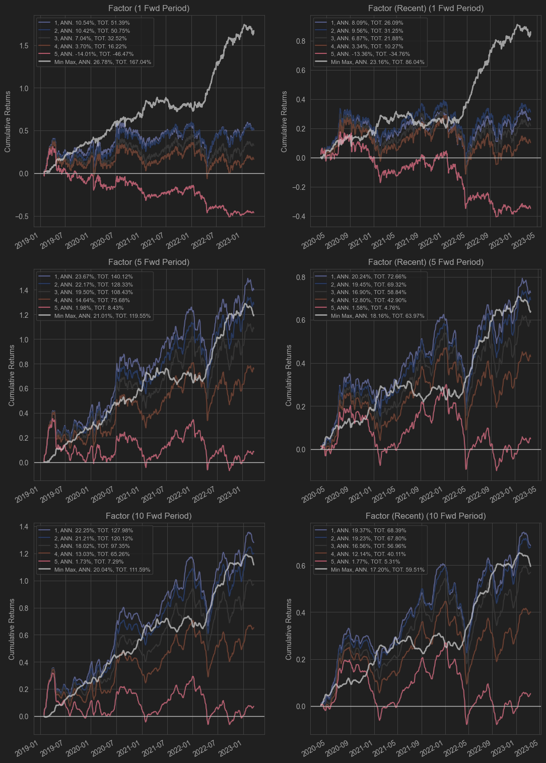
This figure shows the factor’s quantile returns.

The top, middle, and bottom regions correspond to the 1-, 5-, and 10-day return charts, respectively.

The left side shows the return curves for the specified period start_date = '2019-01-01', end_date = '2023-03-31'.

The right side shows the return curves for the most recent three years.

Each quantile (five quantiles plus a max-minus-min spread portfolio) is marked in a different color. The top-left of each chart shows the annualized return (ANN) and the total return over the backtest period.

Other Functions

Compute Forward Return

compute_forward_returns function

Used to compute forward returns for assets under different holding periods.

Computes forward returns for specified holding periods
Supports multiple holding periods (e.g., 1, 5, 10, 20 days)
Uses log returns and then converts to simple returns

# Compute quantile returns for a value factor
value_factor = calculate_value_factor()  # assume this computes the value factor
forward_returns = compute_forward_returns(close_prices, [1, 5, 20])

Compute Quantile Return

compute_quantile_returns function

This is a core function in factor investing, used to compute quantile returns after grouping by factor values. Functionality:

Group factor values into quantiles (5-quantile by default)
Compute the average return for each quantile
Supports weighting (e.g., market-cap weighting)
Supports multiple holding periods

# 5-quantile analysis
quantile_returns = compute_quantile_returns(value_factor, forward_returns, quantiles=5)

# 10-quantile analysis (more granular)
quantile_returns_10 = compute_quantile_returns(value_factor, forward_returns, quantiles=10)

# View the return spread between the highest and lowest quantiles
high_low_spread = quantile_returns[1][5] - quantile_returns[1][1]

Industrial applications:

Factor stratification analysis: compare performance of high-factor vs. low-factor stocks
Long–short strategy construction: build long-short portfolios
Factor efficacy evaluation: judge predictive power via quantile return spreads

`Winsorizer` Class

An important tool for handling outliers, widely used in financial data preprocessing.

`MAD_winsorization` — Median Absolute Deviation (MAD) Method

Description:

Uses median absolute deviation (MAD) to identify outliers
More robust than the mean–standard deviation method; less sensitive to extreme values

# Handle outliers using the MAD method
cleaned_factor = Winsorizer.MAD_winsorization(factor_exposure, scaled=True, k=3)

Industrial applications:

Handling outliers in financial data
Data cleaning before factor standardization
Outlier processing in risk models

`sigma_winsorization` — K-σ Rule

Description:

Uses mean ± K×standard deviation as truncation bounds
A classic statistical outlier handling method

# 3-sigma rule
cleaned_factor_sigma = Winsorizer.sigma_winsorization(factor_exposure, k=3)

# 2.5-sigma rule (more aggressive)
cleaned_factor_sigma_aggressive = Winsorizer.sigma_winsorization(factor_exposure, k=2.5)

Industrial applications:

Outlier handling for return data
Standardizing factor exposures
Computing risk metrics

`percentile_winsorization` — Percentile Truncation

Description:

Uses specified percentiles as truncation bounds
The most straightforward outlier handling method

Key parameters:

percentile: truncation percentiles, default (0.01, 0.99)
set_outlier_nan: whether to set outliers to NaN

# Truncate at the 1% and 99% percentiles
cleaned_factor_percentile = Winsorizer.percentile_winsorization(
    factor_exposure, 
    percentile=(0.01, 0.99)
)

# Truncate at the 5% and 95% percentiles (more conservative)
cleaned_factor_percentile_conservative = Winsorizer.percentile_winsorization(
    factor_exposure, 
    percentile=(0.05, 0.95)
)

# Set outliers to NaN instead of truncating
cleaned_factor_nan = Winsorizer.percentile_winsorization(
    factor_exposure, 
    percentile=(0.01, 0.99),
    set_outlier_nan=True
)

Industrial applications:

Standardizing factor data
Data cleaning before portfolio construction
Outlier handling in backtesting systems

Evaluation of Industrial Factors

Typical Workflow (copy-paste ready)

Step 0. Prepare Two Types of Data

Step 1. Use eva_utils to Compute “Forward Returns” and Understand IC/Quantiles

Step 2. Prepare the Factor (T×N)

Step 3. One-Click Evaluation

Other Functions

Compute Forward Return

Compute Quantile Return

Winsorizer Class

MAD_winsorization — Median Absolute Deviation (MAD) Method

sigma_winsorization — K-σ Rule

percentile_winsorization — Percentile Truncation

Step 1. Use `eva_utils` to Compute “Forward Returns” and Understand IC/Quantiles

`Winsorizer` Class

`MAD_winsorization` — Median Absolute Deviation (MAD) Method

`sigma_winsorization` — K-σ Rule

`percentile_winsorization` — Percentile Truncation